
When it comes to Google Sheets vs Excel, many people choose Google Sheets because it’s free or cheaper than Excel and because it offers enough features to satisfy even spreadsheet power users.
But even if you’ve been using Google Sheets for a while, you may not know all the tricks and tips for getting more done in less time. This post covers 8 Google Sheets productivity hacks you can use to streamline your workload better organize your data.
The Complete List of Google Sheet Productivity Hacks
The following Google Sheets productivity hacks are not arranged in any particular order but generally move from simpler techniques to more complex ones.
Google Sheets is powerful software and there are many things it can do that we didn’t include on this list.
What you’ll find below are some of the most important tips any user can apply to supercharge their productivity when working with Google Sheets.
1. Keyboard Shortcuts
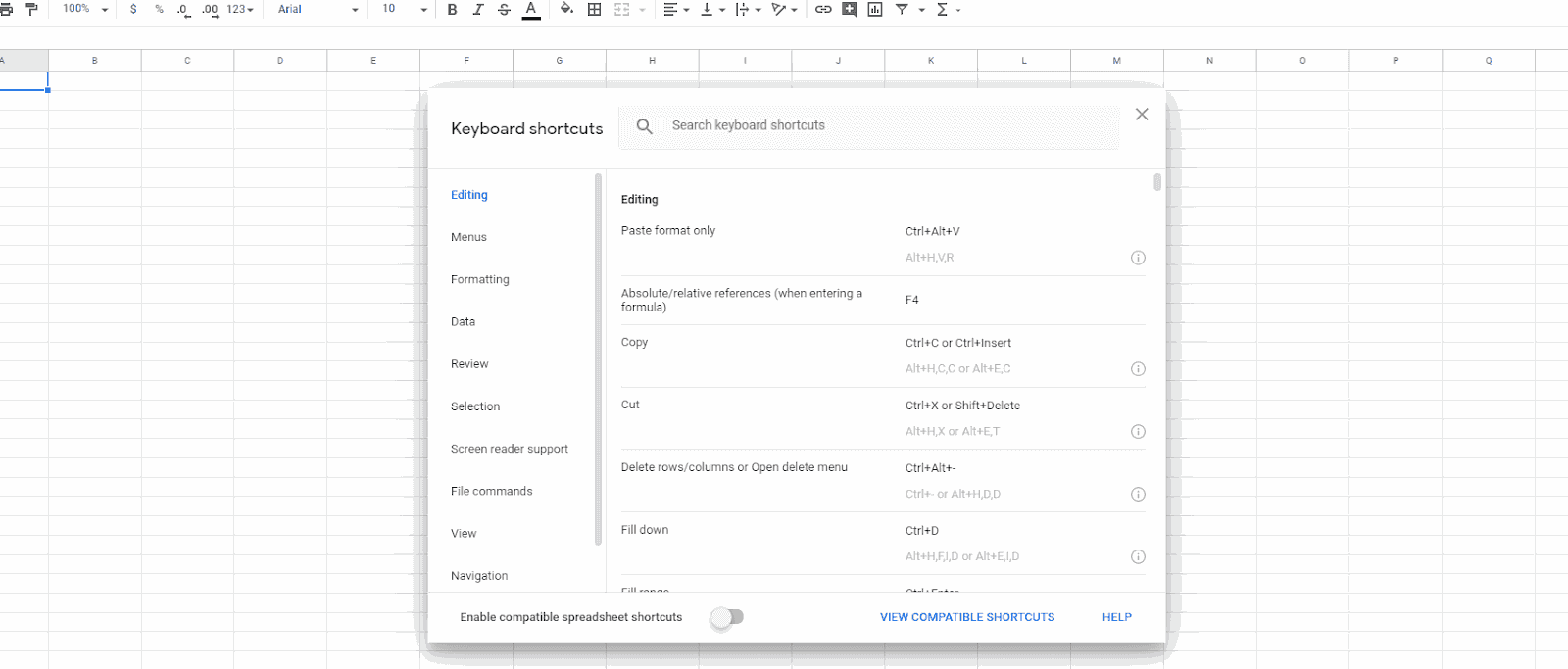
Keyboard shortcuts are the quintessential “hack” and Google Sheets has plenty that you should know. The first one you should know about helps you access the full list of keyboard shortcuts within Google Sheets itself.
If you’re using Apple, hold Command and “forward slash.”
If you’re using Windows, hold Ctrl and “forward slash.”
A popup should appear with a LOOONG list of keyboard shortcuts. Don’t feel overwhelmed. On the left-hand side of this popup will be categories for the keyboard shortcuts:
- Editing
- Menus
- Formating
- Data
- Review
You can click any of these to be taken to the specific shortcuts in that category.
Some that we recommend are:
Clear All Formatting in a cell or range
- Apple: ⌘ +
- Windows: Ctrl +
Insert the current date in a cell
- Apple: ⌘ + ;
- Windows: Ctrl + ;
Find and Replace
- Apple: ⌘ + Shift + H
- Windows: Ctrl + H
Plus, Google Sheets released a few exciting updates to their shortcuts last May. You can now “enable compatible spreadsheet shortcuts” and use common keyboard shortcuts from other spreadsheet software like Excel within Google Sheets.
This added feature makes switching to Google Sheets that much easier.
2. Comment on Cells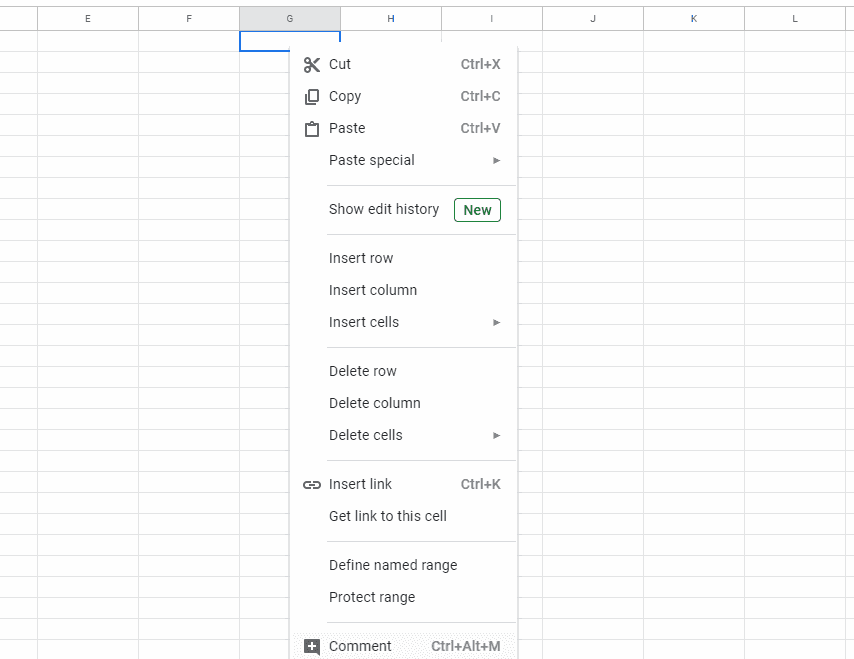
Remote team communication is happening more than ever today, and one of the most important features Google Sheets offers is the ability to leave comments on specific cells.
There are 3 ways to leave a comment in cells:
- Right-click on a specific cell and choose “Comment” from the menu.
- Left-click on a cell then click “Insert” from the Google Sheets menu and select “Comment.”
- Left-click on a cell and enter keyboard shortcut Ctrl + Alt + M (Apple users enter
When you leave a comment, a small yellow triangle will appear in the upper right-hand side of the cell. This makes sure that if anyone checks the spreadsheet, they’ll notice a comment was left.
But you can also leave a specific comment for a specific person and let Google Sheets notify them that they were tagged in a comment.
To do this, type the “@” symbol followed by their email address.
An example comment tagging someone would look like this: “Hey @karenR@gmail.com have you seen this?”
Instead of sending a long, complicated explanation in an email, you can tag teammates and show them what you’re talking about – streamlining communication.
3. Conditional Formatting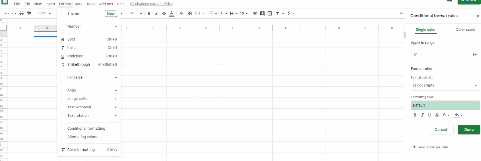
Conditional formatting is a feature that every spreadsheet software has to have, and Google Sheets lets you take advantage of this key function.
Conditional formatting changes the text or background color of cells, rows, or columns based on predefined criteria that you set.
It’s extremely helpful in visualizing data and breaking up the monotony of black letters on white background. You’re less likely to commit errors using conditional formatting because it organizes and arranges data for quick understanding.
To use conditional formatting, highlight all the cells you want to format, navigate to the menu in Google Sheets and select “Format,” then click on “Conditional Formatting.”
A window will pop up on the right-hand side of your screen and let you create as many “rules” as you would like to format your spreadsheet.
4. Add Images to Google Sheets
Spreadsheets are known for collecting all the text and numerical data you can input, but Google Sheets lets you add images as well.
This is helpful if you’re using spreadsheets to track brands (and need their logos), competitor products (if you’re conducting a competitive analysis), or any other images you may need to track alongside other data.
There are two ways to do this:
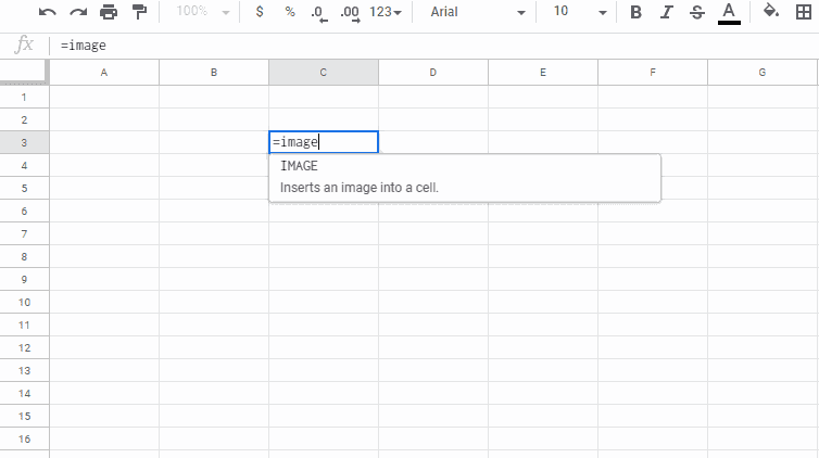
- Left-click on a cell and select “Insert” in the menu and then scroll the cursor over “Image” and select “Image in cell.”
- Left-click on a cell and type the formula =image then paste the link to the image in quotation marks within a pair of parenthesis. Ie. =image (“link”)
When you select “Insert” from the menu and scroll over “Image” you’ll get another option that says “Image over cells.” This lets you paste an image that free-floats above the cells in your spreadsheet that you can freely move.
5. Group Cells In Order
Rarely do spreadsheets contain random information. You’re using Google Sheets to organize information, not spill it out.
Most often, you’ll need to arrange data in a particular order.
For this, you can use the ARRAYFORMULA().
An array is simply a table of values.
The ARRAYFORMULA() processes your data in a single batch. With it, you’re able to make changes to a single cell and have it ripple through the rest of the data range.
The formula is =ARRAYFORMULA(array_formula).
Where it says array_formula, you’ll place either a range of cells, a mathematical expression using one cell range or multiple ranges of the same size, or a function that returns a result greater than one cell.
Here’s an example from Ben L. Collins:

6. Pivot Tables
A basic spreadsheet has rows going horizontally and columns going vertically. If you’re inputting a lot of data over a long period of time, it will become difficult to measure and understand it all.
A pivot table is a tool to summarize and aggregate data to see it in more than just 2 dimensions.
The best way to explain it is to show you how it works.
Take this set of data provided by Google:
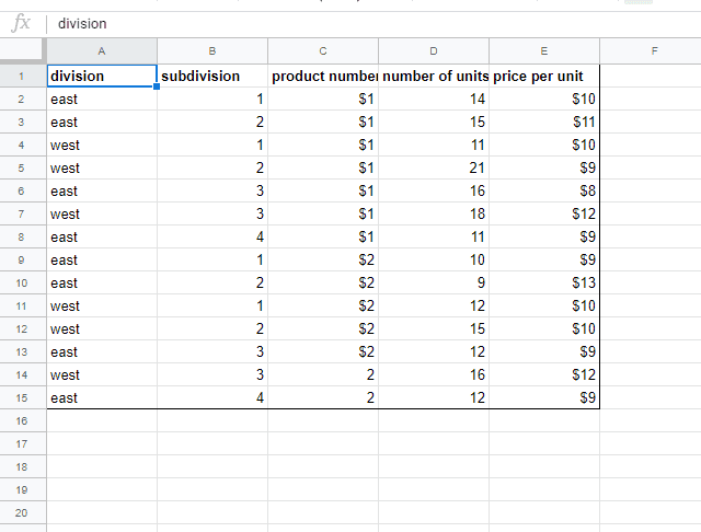
This is a pretty standard spreadsheet for organizing basic inputs for products. The larger this list grows, the more difficult it will be to manage.
To turn this data into a pivot table, highlight all of it and then select “Data” from the menu and click on “Pivot table.” A popup will appear asking if you want to create a new sheet, select that option and press “Create.”
Your pivot table will look something like this:
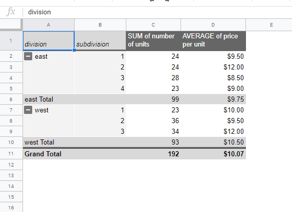
Now instead of a confusing list of inputs, you have a well-organized table summarizing and automatically categorizing the data.
7. Data Validation
Sometimes you may want to ensure certain cells only contain a specific kind of information. If you have a column for sales numbers, you may need to block someone from inputting words or symbols into those cells.
Data validation restricts what values are allowed to be entered into cells.
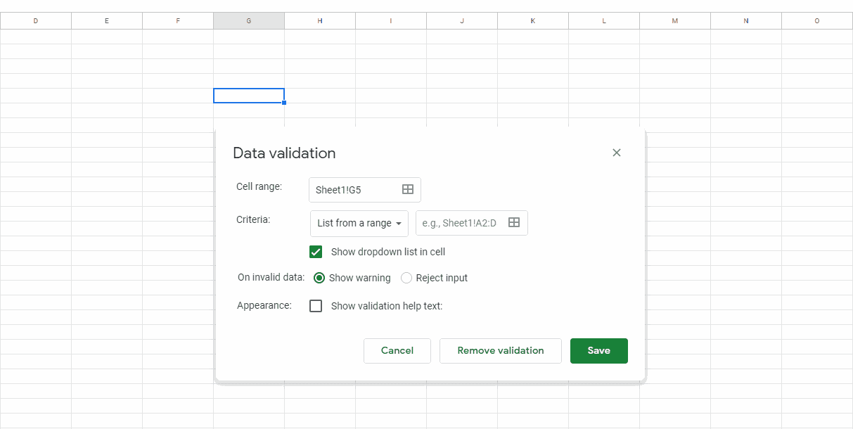
Select all the cells you want to constrain to certain values, click on “Data” in the menu and select “Data validation”
Based on the settings you prefer, you can allow Google Sheets to show a warning when incorrect data is entered or outright reject the input.
You can go one step further and select the option “show validation help text” to display a friendly message informing someone how to input the correct data if they enter the wrong information.
8. Automate Tasks
Repetitively entering the same information over and over again is not only mind-numbing, but it can also lead to harmful errors.
Google Sheets allows you to automate simple tasks using the “Macro” feature.
It records specific actions you take within a spreadsheet and saves the entire process so you can repeat it endlessly in the same sheet or an infinite number of new ones with the click of your mouse or the pressing of a few hotkeys.
To create a Macro, click on “Tools” from the Google Sheets menu, hover your mouse over “Macros” and select “Record Macro.”
You’ll be given a choice to either record a macro using “absolute references” or “relative references.”
Absolute references means that whatever you input into specific cells, the macro will always record the same data in those same cells.
Relative references means that you can enter data into cells, and this macro can be reproduced on any cells you later select.
When you finish recording your macro and click “Save,” you’ll be able to name the saved macro and create a keyboard shortcut to execute the macro at any time.
Bonus Tips to Enhance Your Google Sheets Productivity
- Explore Google Sheets Add-ons Google Sheets has a wide array of add-ons that can significantly extend its functionality. To access them, click on “Extensions” in the menu and then “Add-ons.” You can search for add-ons that help with tasks such as data analysis, visualization, form creation, and more. Popular add-ons include Supermetrics for marketing analytics and Advanced Find and Replace for more robust search functions.
- Use the QUERY Function The QUERY function is an incredibly powerful tool that allows you to run SQL-like queries on your data. This function can filter, sort, and aggregate your data in complex ways without the need for multiple steps. For example, you can use it to quickly summarize sales data by region or by product category.
plaintextCopy code=QUERY(data, "SELECT A, SUM(B) WHERE C='East' GROUP BY A") - Leverage Google Apps Script Google Apps Script lets you automate workflows and create custom functions in Google Sheets. With a bit of JavaScript knowledge, you can write scripts to automate repetitive tasks, create complex data manipulations, or integrate with other Google services.
javascriptCopy codefunction sendEmails() { var sheet = SpreadsheetApp.getActiveSpreadsheet().getSheetByName('Sheet1'); var data = sheet.getDataRange().getValues(); for (var i = 1; i < data.length; i++) { MailApp.sendEmail(data[i][1], 'Subject', 'Email body'); } } - Use Explore for Quick Insights The Explore feature in Google Sheets uses machine learning to provide quick insights into your data. You can access it by clicking the small star icon in the bottom right corner of your sheet. Explore can help you generate charts, find patterns, and even suggest formulas based on your data.
- Create Dropdown Lists Dropdown lists can make data entry faster and more consistent. To create a dropdown list, select the cells where you want the list to appear, then click on “Data” and select “Data validation.” Choose “List of items” or “List from a range” and enter your options.
- Split Text into Columns If you have a column of data that contains multiple pieces of information (e.g., full names), you can split this data into separate columns. Highlight the column, then go to “Data” and select “Split text to columns.” Choose your delimiter (e.g., space, comma) and Google Sheets will separate the data accordingly.
- Protect Ranges and Sheets To prevent accidental edits, you can protect specific ranges or entire sheets. Select the range or sheet you want to protect, right-click, and choose “Protect range.” You can then set permissions to limit who can edit the protected areas.
- Utilize Import Functions Google Sheets allows you to import data from other sheets, websites, or even databases using functions like
IMPORTRANGE,IMPORTHTML, andIMPORTDATA. These functions can keep your data up-to-date by pulling the latest information from external sources.
plaintextCopy code=IMPORTRANGE("https://docs.google.com/spreadsheets/d/abc123", "Sheet1!A1:D10") - Use Conditional Sum and Count Functions like
SUMIF,COUNTIF,AVERAGEIF, and their plural counterparts (SUMIFS,COUNTIFS,AVERAGEIFS) are extremely useful for conditional calculations. These functions help you perform calculations based on specific criteria within your data.
plaintextCopy code=SUMIF(A:A, "East", B:B) - Embed Google Sheets in Docs or Slides You can embed charts or data from Google Sheets directly into Google Docs or Slides, ensuring that your presentations and reports always reflect the most current data. Simply copy the chart or range in Google Sheets, then paste it into your Doc or Slide and choose the “Link to spreadsheet” option.
Conclusion
By incorporating these additional tips into your Google Sheets workflow, you can further streamline your processes, enhance collaboration, and make data management more efficient. Whether you’re automating repetitive tasks, using advanced functions, or leveraging add-ons, these techniques will help you get the most out of Google Sheets.
4o
How to Boost Team Collaboration When Using Google Sheets
The data collected in Google Sheets (and organized using the productivity hacks on this list) will most likely be shared with one or more members of your team.
However, these team members may need more help in understanding the data or specific processes you used to compile it.
Instead of typing up explanations or trying to talk them through it, you can use different visual communication tactics to clarify their confusion.
You can turn a certain process into a GIF.
Annotate screenshots of the data to illuminate its meaning.
Or record a webcam where you demonstrate your calculations or present the data so that your team members can see it while you discuss it.
Zight (formerly CloudApp) gives you these options and plenty more.
We’ve been ranked by G2 Crowd as one of the top sales enablement tools and can help you be more productive by communicating better.
Find out why Zight (formerly CloudApp) should be paired with Google Sheets productivity hacks for enhanced teamwork today.